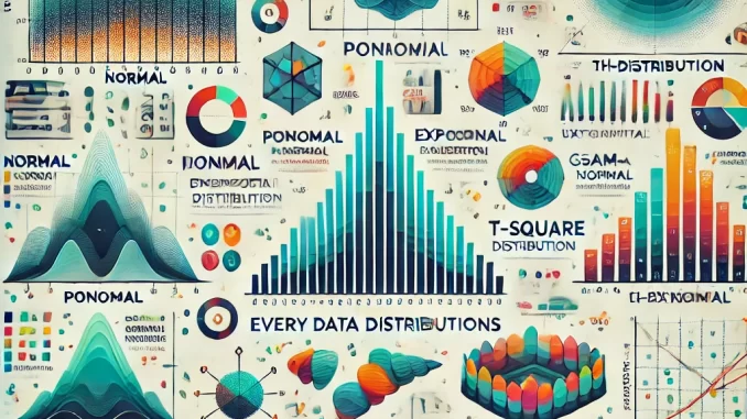
Statistical Distributions Every Data Scientist Should Know
In the realm of data science, understanding statistical distributions is crucial for extracting meaningful insights, building predictive models, and interpreting results effectively. Statistical distributions describe how values are distributed within a dataset and underpin many algorithms and analytical techniques. Here are the key statistical distributions every data scientist should know:
1. Normal Distribution
Also known as the Gaussian distribution, the normal distribution is ubiquitous in statistics and data science. It’s characterized by its bell-shaped curve and symmetry about the mean. Key properties include:
- Parameters: Mean (μ) and standard deviation (σ).
- Applications: Many natural phenomena (e.g., heights, test scores) follow a normal distribution. Central Limit Theorem also states that the sampling distribution of the mean tends to be normal for large sample sizes.
2. Binomial Distribution
The binomial distribution models the number of successes in a fixed number of independent Bernoulli trials.
- Parameters: Number of trials (τ) and probability of success (p).
- Applications: Predicting outcomes like coin tosses, customer purchases, or email clicks.
3. Poisson Distribution
The Poisson distribution describes the number of events occurring within a fixed interval of time or space when these events occur independently.
- Parameters: Average rate of occurrence (λ).
- Applications: Modeling rare events like server downtimes, customer arrivals, or website hits per hour.
4. Exponential Distribution
Often associated with the Poisson distribution, the exponential distribution models the time between successive events.
- Parameters: Rate parameter (λ).
- Applications: Used in survival analysis, reliability engineering, and queuing theory to model lifetimes of devices or wait times.
5. Uniform Distribution
The uniform distribution is characterized by an equal probability for all outcomes within a specific range.
- Parameters: Lower bound (a) and upper bound (b).
- Applications: Simulating random variables and generating synthetic datasets.
6. Chi-Square Distribution
The chi-square distribution is the distribution of the sum of squared standard normal variables and is used extensively in hypothesis testing.
- Parameters: Degrees of freedom (ν).
- Applications: Goodness-of-fit tests, tests for independence, and confidence intervals for variance.
7. Student’s t-Distribution
The t-distribution is similar to the normal distribution but has heavier tails, making it suitable for small sample sizes.
- Parameters: Degrees of freedom (ν).
- Applications: Confidence intervals and hypothesis tests for small datasets where the population standard deviation is unknown.
8. Gamma Distribution
The gamma distribution generalizes the exponential distribution and models waiting times for multiple events to occur.
- Parameters: Shape parameter (α) and rate parameter (β).
- Applications: Used in Bayesian statistics and queuing models.
9. Beta Distribution
The beta distribution is a continuous distribution defined on the interval [0, 1]. It is highly flexible due to its two shape parameters.
- Parameters: α and β (shape parameters).
- Applications: Bayesian analysis and modeling probabilities.
10. Log-Normal Distribution
A variable follows a log-normal distribution if its logarithm is normally distributed.
- Parameters: Mean and standard deviation of the variable’s natural logarithm.
- Applications: Modeling skewed data like stock prices or income levels.
Why Understanding Distributions Matters
- Model Assumptions: Many machine learning algorithms and statistical tests rely on specific distributional assumptions.
- Data Generation: Simulating realistic data for testing models.
- Feature Engineering: Identifying appropriate transformations for non-normal data.
- Anomaly Detection: Identifying outliers using statistical thresholds.
Tools to Explore Distributions
Data scientists can use tools like Python libraries (e.g., NumPy, SciPy, matplotlib, seaborn) and R packages to visualize and analyze distributions. For example:
import numpy as np
import seaborn as sns
import matplotlib.pyplot as plt

# Example: Visualizing a normal distribution
mean = 0
std_dev = 1
data = np.random.normal(mean, std_dev, 1000)
sns.histplot(data, kde=True)
plt.title("Normal Distribution")
plt.show()
Mastering these statistical distributions empowers data scientists to make informed decisions, validate models, and communicate findings effectively. Whether analyzing trends, building predictive models, or deriving actionable insights, a strong foundation in distributions is indispensable for success in data science.

Leave a Reply